End-to-end tutorial - Classification

This should give you an idea on how this library works

In this tutorial, we will use the Pima Indian dataset https://www.kaggle.com/datasets/uciml/pima-indians-diabetes-database. The objective of the dataset is to diagnostically predict whether or not a patient has diabetes, based on certain diagnostic measurements included in the dataset.

from that_ml_library.data_preprocess import *
from that_ml_library.chart_plotting import *
from that_ml_library.ml_helpers import *

Load data

import pandas as pd
import numpy as np

df = pd.read_csv('https://raw.githubusercontent.com/anhquan0412/dataset/main/diabetes.csv')
print(df.shape)
display(df.sample(7))

(768, 9)

	Pregnancies	Glucose	BloodPressure	SkinThickness	Insulin	BMI	DiabetesPedigreeFunction	Age	Outcome
92	7	81	78	40	48	46.7	0.261	42	0
54	7	150	66	42	342	34.7	0.718	42	0
288	4	96	56	17	49	20.8	0.340	26	0
90	1	80	55	0	0	19.1	0.258	21	0
98	6	93	50	30	64	28.7	0.356	23	0
397	0	131	66	40	0	34.3	0.196	22	1
574	1	143	86	30	330	30.1	0.892	23	0

df.info()

<class 'pandas.core.frame.DataFrame'>
RangeIndex: 768 entries, 0 to 767
Data columns (total 9 columns):
 #   Column                    Non-Null Count  Dtype  
---  ------                    --------------  -----  
 0   Pregnancies               768 non-null    int64  
 1   Glucose                   768 non-null    int64  
 2   BloodPressure             768 non-null    int64  
 3   SkinThickness             768 non-null    int64  
 4   Insulin                   768 non-null    int64  
 5   BMI                       768 non-null    float64
 6   DiabetesPedigreeFunction  768 non-null    float64
 7   Age                       768 non-null    int64  
 8   Outcome                   768 non-null    int64  
dtypes: float64(2), int64(7)
memory usage: 54.1 KB

Train test split and preprocessing

from sklearn.model_selection import train_test_split

X_train, X_test, y_train, y_test = train_test_split(df.iloc[:,:-1], df.Outcome,
                                                    test_size=0.2,
                                                    random_state=42,
                                                    stratify=df.Outcome)

X_train.describe()

	Pregnancies	Glucose	BloodPressure	SkinThickness	Insulin	BMI	DiabetesPedigreeFunction	Age
count	614.000000	614.000000	614.000000	614.000000	614.000000	614.000000	614.000000	614.000000
mean	3.819218	120.908795	69.442997	20.776873	78.666124	31.973290	0.477428	33.366450
std	3.314148	31.561093	18.402581	15.856433	107.736572	7.861364	0.330300	11.833438
min	0.000000	0.000000	0.000000	0.000000	0.000000	0.000000	0.084000	21.000000
25%	1.000000	99.000000	62.500000	0.000000	0.000000	27.500000	0.245000	24.000000
50%	3.000000	117.000000	72.000000	23.000000	40.500000	32.300000	0.382500	29.000000
75%	6.000000	140.000000	80.000000	32.000000	130.000000	36.500000	0.639250	41.000000
max	17.000000	199.000000	122.000000	99.000000	744.000000	67.100000	2.329000	81.000000

For this dataset, we only need to perform scaling on numerical features, as there’s no categorical features to process. Note that scaling of numerical data is required for linear model such as linear regression, and not required for tree model, though it doesn’t hurt the performance of such tree model. For simplicity, we will scale the numerical features for all the models we are going to run below.

num_cols = df.columns[:-1].tolist()
print(num_cols)

['Pregnancies', 'Glucose', 'BloodPressure', 'SkinThickness', 'Insulin', 'BMI', 'DiabetesPedigreeFunction', 'Age']

For Blood Pressure and Skin Thickness, a value of 0 does not make sense, so we will consider these as missing values. The strategy for filling in the missing values will be ‘median’

miss_cols = ['BloodPressure','SkinThickness']

X_train_processed,X_test_processed = preprocessing_general(X_train,X_test,
                                                           miss_cols=miss_cols,
                                                           missing_vals=0,strategies='median',
                                                           num_cols=num_cols,
                                                           scale_methods='minmax')

X_train_processed.describe()

	Pregnancies	Glucose	BloodPressure	SkinThickness	Insulin	BMI	DiabetesPedigreeFunction	Age
count	614.000000	614.000000	614.000000	614.000000	614.000000	614.000000	614.000000	614.000000
mean	0.224660	0.607582	0.569205	0.209867	0.105734	0.476502	0.175246	0.206107
std	0.194950	0.158598	0.150841	0.160166	0.144807	0.117159	0.147127	0.197224
min	0.000000	0.000000	0.000000	0.000000	0.000000	0.000000	0.000000	0.000000
25%	0.058824	0.497487	0.512295	0.000000	0.000000	0.409836	0.071715	0.050000
50%	0.176471	0.587940	0.590164	0.232323	0.054435	0.481371	0.132962	0.133333
75%	0.352941	0.703518	0.655738	0.323232	0.174731	0.543964	0.247327	0.333333
max	1.000000	1.000000	1.000000	1.000000	1.000000	1.000000	1.000000	1.000000

Machine Learning Model Experiments

from sklearn.model_selection import StratifiedKFold

cv = StratifiedKFold(5)

Sklearn Logistic Regression

df_train = X_train_processed.copy()
df_train['has_diabetes'] = y_train

get_vif(df_train,plot_corr=True)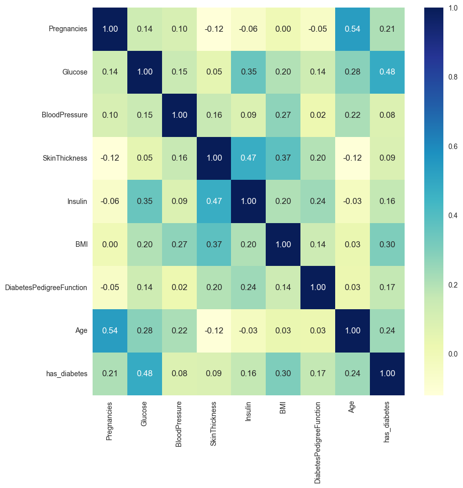

const                       40.937975
Pregnancies                  1.441405
Glucose                      1.573457
BloodPressure                1.152426
SkinThickness                1.529585
Insulin                      1.538192
BMI                          1.343058
DiabetesPedigreeFunction     1.097619
Age                          1.577323
has_diabetes                 1.451467
dtype: float64

With VIF, we can see that there’s not much colinearity in this dataset. Note that VIF >5 or >10 means high colinearity

run_logistic_regression(X_train_processed,y_train,
                        multi_class='multinomial',
                        solver='newton-cg',max_iter=10000)

	Features	Coefficients	Coefficients Exp
0	Intercept	-4.233888	0.014496
1	Pregnancies	0.976679	2.655623
2	Glucose	3.679170	39.613487
3	BloodPressure	-0.679500	0.506870
4	SkinThickness	0.217158	1.242540
5	Insulin	-0.473694	0.622698
6	BMI	3.106698	22.347132
7	DiabetesPedigreeFunction	0.881984	2.415688
8	Age	0.461467	1.586400

----------------------------------------------------------------------------------------------------
Log loss:  0.46620685663024525
----------------------------------------------------------------------------------------------------
              precision    recall  f1-score   support

           0       0.81      0.90      0.85       400
           1       0.76      0.60      0.67       214

    accuracy                           0.79       614
   macro avg       0.78      0.75      0.76       614
weighted avg       0.79      0.79      0.79       614

LogisticRegression(max_iter=10000, multi_class='multinomial', penalty=None,
                   random_state=0, solver='newton-cg')

In a Jupyter environment, please rerun this cell to show the HTML representation or trust the notebook.
On GitHub, the HTML representation is unable to render, please try loading this page with nbviewer.org.

Interpretation of coefficients in logistic regression: For a coefficient β1, given a one unit increase in one of the variables (say X1), the odds of X (p(X)/1-p(X)) will be multiplied by e^β1.

In this case, we can tell from coefficient of Glucose that: the odd of having diabetes will be multiplied by ~40 if Glucose level is increased by 1

Statsmodel

run_multinomial_statmodel(X_train_processed,y_train,add_constant=True)

Optimization terminated successfully.
         Current function value: 0.466207
         Iterations 6
                          MNLogit Regression Results                          
==============================================================================
Dep. Variable:                Outcome   No. Observations:                  614
Model:                        MNLogit   Df Residuals:                      605
Method:                           MLE   Df Model:                            8
Date:                Mon, 19 Feb 2024   Pseudo R-squ.:                  0.2789
Time:                        11:43:30   Log-Likelihood:                -286.25
converged:                       True   LL-Null:                       -396.97
Covariance Type:            nonrobust   LLR p-value:                 1.909e-43
============================================================================================
               Outcome=1       coef    std err          z      P>|z|      [0.025      0.975]
--------------------------------------------------------------------------------------------
const                       -8.4678      0.805    -10.523      0.000     -10.045      -6.891
Pregnancies                  1.9534      0.624      3.129      0.002       0.730       3.177
Glucose                      7.3584      0.855      8.609      0.000       5.683       9.034
BloodPressure               -1.3590      0.733     -1.855      0.064      -2.795       0.077
SkinThickness                0.4343      0.788      0.551      0.581      -1.110       1.978
Insulin                     -0.9474      0.856     -1.107      0.268      -2.625       0.730
BMI                          6.2135      1.150      5.405      0.000       3.960       8.467
DiabetesPedigreeFunction     1.7640      0.755      2.335      0.020       0.283       3.245
Age                          0.9229      0.616      1.499      0.134      -0.284       2.130
============================================================================================
----------------------------------------------------------------------------------------------------
Log loss:  0.46620685662395556
----------------------------------------------------------------------------------------------------
              precision    recall  f1-score   support

           0       0.81      0.90      0.85       400
           1       0.76      0.60      0.67       214

    accuracy                           0.79       614
   macro avg       0.78      0.75      0.76       614
weighted avg       0.79      0.79      0.79       614

<statsmodels.discrete.discrete_model.MNLogit>

Decision Tree

Validation Curve

from sklearn.tree import DecisionTreeClassifier

dt = DecisionTreeClassifier(criterion='entropy',random_state=42,class_weight=None)
cv = StratifiedKFold(5)
plot_validation_curve(dt,'Val Curve - Decision Tree - PID',X_train_processed,y_train,
                      cv=cv,param_range=np.arange(1,20,1),param_name='max_depth',scoring='f1_macro',
                      n_jobs=-1,figsize=(6,4))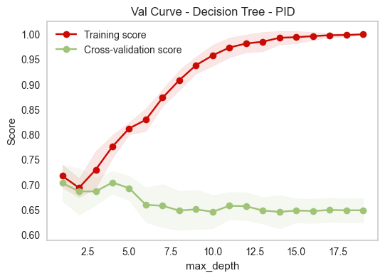

This is the validation curve for hyperparameter max depth, which can be used to prune a decision tree.

For max depth, we can observe the overfitting behavior when max depth is too high, which means the tree is able to make unlimited splits to the extreme of classifying each of the training data points correctly, thus failing to generalize. On the other hand, a small depth is enough to achieve a good CV score (from depth 1 to 5). This is a telling sign that some features have strong signals to predict diabetes than others.

Learning curve

np.linspace(0.1,1,20)

array([0.1       , 0.14736842, 0.19473684, 0.24210526, 0.28947368,
       0.33684211, 0.38421053, 0.43157895, 0.47894737, 0.52631579,
       0.57368421, 0.62105263, 0.66842105, 0.71578947, 0.76315789,
       0.81052632, 0.85789474, 0.90526316, 0.95263158, 1.        ])

dt = DecisionTreeClassifier(criterion='entropy',random_state=42,class_weight=None,min_samples_leaf=27)
plot_learning_curve(dt,'DT Learning Curve',X_train_processed,y_train,cv=cv,scoring='f1_macro',
                    train_sizes=np.linspace(0.1,1,20))

Based on the learning curve for the best tuned decision tree, more data is better for the model to learn, as training score seems to convert, and CV score still slowly increases. However, as the gap between CV score and train score is closing, adding lots of data might not be beneficial. For the scalability of the model, the relationship between training time and fit time is linear, which makes sense as more data allows tree to grow more, which takes more time to fit and predict.

Tree plotting

Using Dtreeviz

dt = DecisionTreeClassifier(criterion='entropy',random_state=42,class_weight=None,max_depth=3)
dt.fit(X_train_processed,y_train)
plot_tree_dtreeviz(dt,X_train_processed,y_train,target_name='has_diabetes',class_names=['no','yes'],
                   fancy=True,scale=1.0)

/home/quan/anaconda3/envs/dev/lib/python3.10/site-packages/sklearn/base.py:439: UserWarning: X does not have valid feature names, but DecisionTreeClassifier was fitted with feature names

Glucose alone can make CV F1 score to reach 0.704, which is not far from the CV score of the best tuned model. With domain knowledge, we can confirm that high glucose is the number one indicator for diabetes, because diabetes patients are unable to effectively use insulin to break down glucose.

Using Sklearn tree plot

dt = DecisionTreeClassifier(criterion='entropy',random_state=42,class_weight=None,max_depth=3)
dt.fit(X_train_processed,y_train)
plot_classification_tree_sklearn(dt,feature_names=X_train_processed.columns.values,
                  class_names=['no','yes'],
                  rotate=True,fname='tree_depth_3_PID')

Type 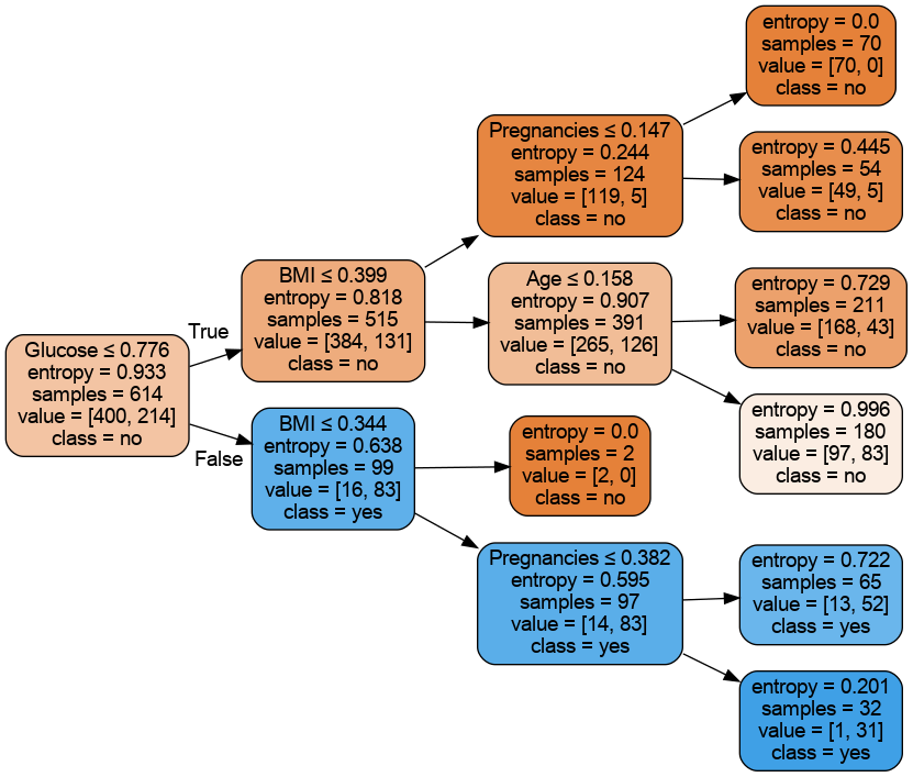![](images/tree_depth_3_PID.png)

Model finetuning process

from sklearn.ensemble import RandomForestClassifier

param_grid = {
    'n_estimators': np.arange(2,80),
    'min_samples_leaf': np.arange(1,100),
    'max_features': [0.3,0.4,0.5,0.6,0.7,0.8,0.9,1],
}
search_cv = tune_sklearn_model('RandomForest',param_grid,X_train_processed,y_train,
                               is_regression=False,
                               custom_cv=5,
                               scoring='f1_macro',
                               random_cv_iter=100,
                               rank_show=7,
                               show_split_scores=True)

Fitting 5 folds for each of 100 candidates, totalling 500 fits
----------
Rank 1
Params: {'n_estimators': 4, 'min_samples_leaf': 23, 'max_features': 0.7}
Train scores: [0.77, 0.76, 0.78, 0.76, 0.78]
Mean train score: 0.768 +- 0.008
Test scores:  [0.73, 0.77, 0.71, 0.7, 0.77]
Mean test score: 0.738 +- 0.029
----------
Rank 2
Params: {'n_estimators': 41, 'min_samples_leaf': 5, 'max_features': 0.5}
Train scores: [0.88, 0.87, 0.86, 0.88, 0.87]
Mean train score: 0.872 +- 0.009
Test scores:  [0.71, 0.78, 0.71, 0.71, 0.77]
Mean test score: 0.737 +- 0.031
----------
Rank 3
Params: {'n_estimators': 31, 'min_samples_leaf': 10, 'max_features': 0.6}
Train scores: [0.83, 0.81, 0.82, 0.82, 0.81]
Mean train score: 0.819 +- 0.011
Test scores:  [0.72, 0.77, 0.7, 0.69, 0.79]
Mean test score: 0.737 +- 0.040
----------
Rank 4
Params: {'n_estimators': 20, 'min_samples_leaf': 28, 'max_features': 0.5}
Train scores: [0.77, 0.76, 0.78, 0.76, 0.78]
Mean train score: 0.770 +- 0.008
Test scores:  [0.75, 0.76, 0.71, 0.68, 0.78]
Mean test score: 0.735 +- 0.037
----------
Rank 5
Params: {'n_estimators': 18, 'min_samples_leaf': 94, 'max_features': 0.7}
Train scores: [0.73, 0.73, 0.74, 0.75, 0.72]
Mean train score: 0.735 +- 0.011
Test scores:  [0.74, 0.76, 0.7, 0.71, 0.77]
Mean test score: 0.735 +- 0.026
----------
Rank 6
Params: {'n_estimators': 35, 'min_samples_leaf': 61, 'max_features': 0.8}
Train scores: [0.74, 0.74, 0.77, 0.75, 0.73]
Mean train score: 0.746 +- 0.011
Test scores:  [0.8, 0.76, 0.69, 0.67, 0.76]
Mean test score: 0.734 +- 0.045
----------
Rank 7
Params: {'n_estimators': 35, 'min_samples_leaf': 8, 'max_features': 0.5}
Train scores: [0.84, 0.82, 0.83, 0.84, 0.82]
Mean train score: 0.832 +- 0.008
Test scores:  [0.75, 0.76, 0.7, 0.71, 0.76]
Mean test score: 0.734 +- 0.027
----------
Default Params
Mean train score: 1.0 +- 0.0
Mean test score: 0.731 +- 0.04

[Parallel(n_jobs=-1)]: Using backend LokyBackend with 24 concurrent workers.
[Parallel(n_jobs=-1)]: Done   5 out of   5 | elapsed:    0.2s finished

params_3D_heatmap(search_cv,'n_estimators','min_samples_leaf','max_features','f1_macro')

By looking at the 3D map of these three hyperparameters, we might need to exclude max_features of 1 and min_samples_leaf that is more than 80. In fact, max_features of 0.8 and 0.9 shows the most promising set of hyperparameters, thus we can now simplied our search space to this:

param_grid = {
    'n_estimators': np.arange(2,80),
    'min_samples_leaf': np.arange(1,85),
    'max_features': [0.8,0.9],
}
search_cv = tune_sklearn_model('RandomForest',param_grid,X_train_processed,y_train,custom_cv=5,
                               scoring='f1_macro',
                               random_cv_iter=200,
                               rank_show=2,
                               show_split_scores=True)

Fitting 5 folds for each of 200 candidates, totalling 1000 fits
----------
Rank 1
Params: {'n_estimators': 12, 'min_samples_leaf': 12, 'max_features': 0.8}
Train scores: [0.8, 0.8, 0.81, 0.82, 0.8]
Mean train score: 0.806 +- 0.010
Test scores:  [0.74, 0.79, 0.7, 0.7, 0.79]
Mean test score: 0.743 +- 0.041
----------
Rank 2
Params: {'n_estimators': 33, 'min_samples_leaf': 23, 'max_features': 0.8}
Train scores: [0.78, 0.76, 0.77, 0.77, 0.76]
Mean train score: 0.769 +- 0.007
Test scores:  [0.75, 0.77, 0.71, 0.69, 0.79]
Mean test score: 0.742 +- 0.038
----------
Default Params
Mean train score: 1.0 +- 0.0
Mean test score: 0.731 +- 0.04

[Parallel(n_jobs=-1)]: Using backend LokyBackend with 24 concurrent workers.
[Parallel(n_jobs=-1)]: Done   5 out of   5 | elapsed:    0.2s finished

params_2D_heatmap(search_cv,'n_estimators','min_samples_leaf','f1_macro',
                  figsize=(20,10),min_hm=0.7,max_hm=None)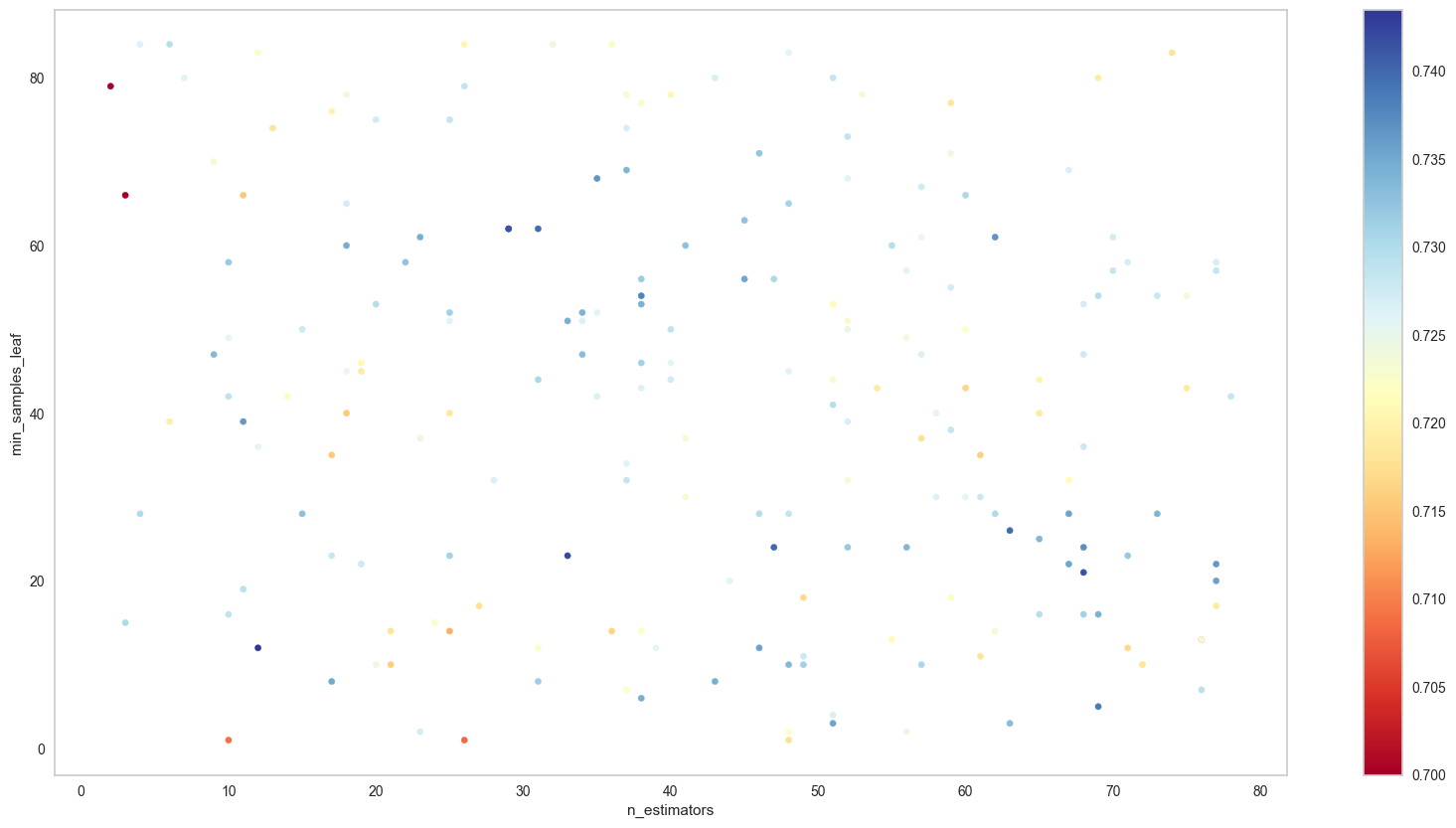

We will now focus on the area near the bottom right of the graph, for grid search

param_grid = {
    'n_estimators': np.arange(62,73),
    'min_samples_leaf': np.arange(20,26),
    'max_features': [0.9],
}
search_cv = tune_sklearn_model('RandomForest',
                              param_grid,
                              X_train_processed,
                              y_train,
                              scoring='f1_macro',
                              custom_cv=5,
                              rank_show=5)

Fitting 5 folds for each of 66 candidates, totalling 330 fits
----------
Rank 1
Params: {'max_features': 0.9, 'min_samples_leaf': 25, 'n_estimators': 72}
Train scores: [0.77, 0.75, 0.78, 0.76, 0.77]
Mean train score: 0.767 +- 0.009
Test scores:  [0.74, 0.78, 0.7, 0.72, 0.78]
Mean test score: 0.745 +- 0.033
----------
Rank 1
Params: {'max_features': 0.9, 'min_samples_leaf': 25, 'n_estimators': 63}
Train scores: [0.78, 0.75, 0.77, 0.77, 0.77]
Mean train score: 0.765 +- 0.009
Test scores:  [0.74, 0.78, 0.7, 0.72, 0.78]
Mean test score: 0.745 +- 0.033
----------
Rank 1
Params: {'max_features': 0.9, 'min_samples_leaf': 25, 'n_estimators': 65}
Train scores: [0.78, 0.75, 0.78, 0.76, 0.77]
Mean train score: 0.766 +- 0.009
Test scores:  [0.74, 0.78, 0.7, 0.72, 0.78]
Mean test score: 0.745 +- 0.033
----------
Rank 1
Params: {'max_features': 0.9, 'min_samples_leaf': 25, 'n_estimators': 62}
Train scores: [0.77, 0.75, 0.77, 0.77, 0.77]
Mean train score: 0.765 +- 0.008
Test scores:  [0.74, 0.78, 0.7, 0.72, 0.78]
Mean test score: 0.745 +- 0.033
----------
Rank 5
Params: {'max_features': 0.9, 'min_samples_leaf': 25, 'n_estimators': 67}
Train scores: [0.78, 0.75, 0.77, 0.76, 0.77]
Mean train score: 0.766 +- 0.011
Test scores:  [0.74, 0.78, 0.7, 0.71, 0.78]
Mean test score: 0.743 +- 0.034
----------
Default Params
Mean train score: 1.0 +- 0.0
Mean test score: 0.731 +- 0.04

[Parallel(n_jobs=-1)]: Using backend LokyBackend with 24 concurrent workers.
[Parallel(n_jobs=-1)]: Done   5 out of   5 | elapsed:    0.2s finished

Feature importance (permutation technique)

params= {'max_features': 0.9, 'min_samples_leaf': 25, 'n_estimators': 62}
# Mean train score: 0.765 +- 0.008
# Mean test score: 0.745 +- 0.033

# # turn off warnings
# def warn(*args, **kwargs):
#     pass
# import warnings
# warnings.warn = warn

final_model= run_sklearn_model('RandomForest',
                                         params,
                                         X_train_processed,y_train,
                                         is_regression=False,
                                         class_names=['no','yes'],
                                         test_split=None,
                                         seed=42,
                                         plot_fea_imp=True)

------------------------------ Train set ------------------------------
Log loss: 0.4134397147185217
              precision    recall  f1-score   support

          no       0.82      0.90      0.86       400
         yes       0.78      0.63      0.70       214

    accuracy                           0.81       614
   macro avg       0.80      0.77      0.78       614
weighted avg       0.80      0.81      0.80       614

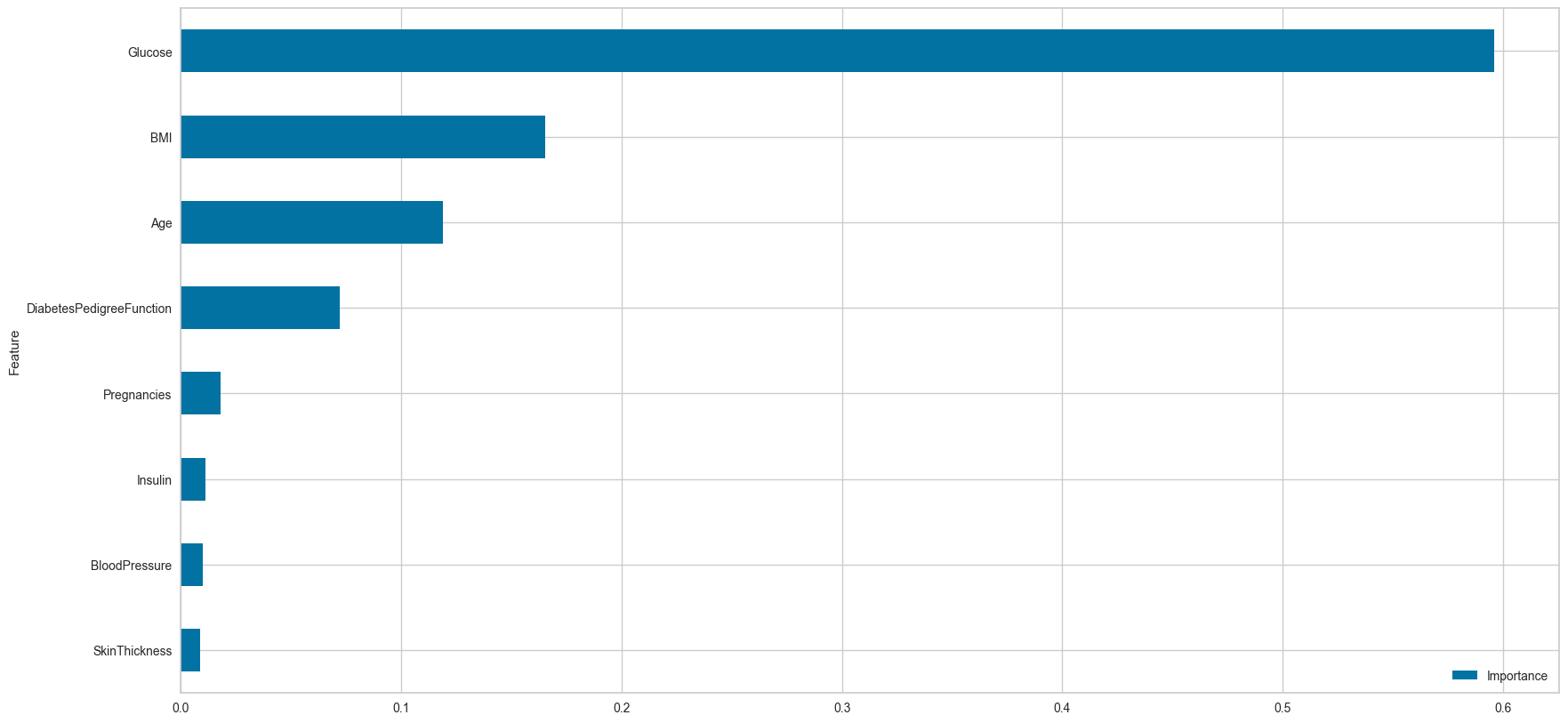
Insulin is not an impact feature for this dataset. Digging deeper on the source of the data, there’s a description that said: “This population has minimal European admixture, and their diabetes appears to be exclusively type 2 diabetes, with no evidence of the autoimmunity characteristic of type 1 diabetes”. Type 2 diabetes patients can still produce insulin, but the body is unable to use it. This information about insulin can be useful later if we want to perform feature selection, in order to boost this model’s performance

Partial Dependency Plot

num_features = X_train_processed.columns.tolist()
num_features

['Pregnancies',
 'Glucose',
 'BloodPressure',
 'SkinThickness',
 'Insulin',
 'BMI',
 'DiabetesPedigreeFunction',
 'Age']

pdp_numerical_only(final_model,X_train_processed,num_features,class_names=['no diabetes','diabetes'],
                  nrows=4,ncols=2)
# y_class is ignored in binary classification or classical regression settings.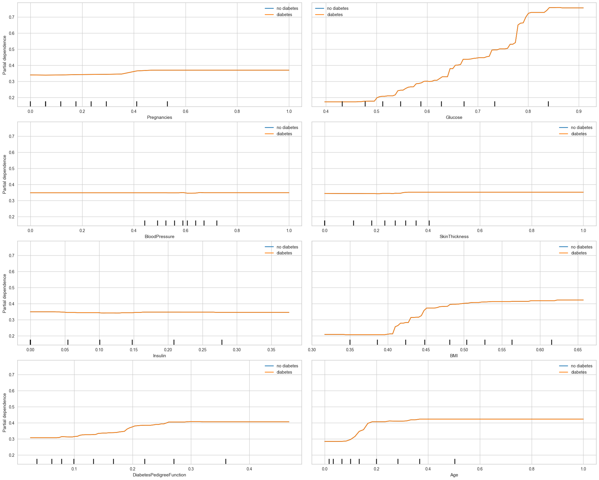

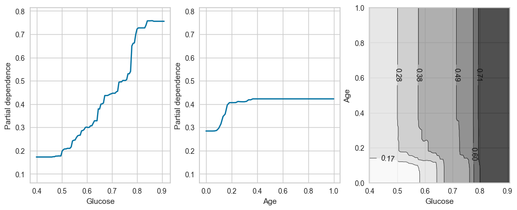
For Partial Dependency Plot, Glucose, BMI and Age show the most changes compared to other features. This matches the feature importances plot earlier.

plot_ice_pair(final_model,X_train_processed,pair_features=['Glucose','Age'],class_idx=1,figsize=(10,4))
# class_idx is ignored in binary classification or classical regression settings.