from that_ml_library.data_preprocess import *
from sklearn.tree import DecisionTreeClassifier
from sklearn.ensemble import RandomForestClassifier,AdaBoostClassifier
from sklearn.preprocessing import LabelEncoderchart_plotting
Variance Inflation Factor and Correlation
get_vif
 get_vif (df:pandas.core.frame.DataFrame, plot_corr=False, figsize=(10,
          10))
*Perform variance inflation factor calculation, and optionally plot correlation matrix
Note that your dataframe should only have numerical features to perform VIF*
| Type | Default | Details | |
|---|---|---|---|
| df | pd.DataFrame | dataframe to plot | |
| plot_corr | bool | False | to plot the correlation matrix |
| figsize | tuple | (10, 10) | Matplotlib figsize |
1. Why you should use VIF: to detect multicollinearity (more than 2 columns)
- Compute variance inflation factor
- The VIF is variance inflation factor the ratio of the variance of βˆj when fitting the full model (with other features) divided by the variance of βˆj if fit on its own
- Min(VIF) = 1 (no collinearity)
- VIF >5 or >10 means high collinearity
2. How to calculating VIF: Set the suspected collinearity feature (e.g. X1) as label, and try to predict X1 using a regression model and other features
3. What to do with high collinearity:
Drop one of them
Combine them to create a new feature
Perform an analysis designed for highly correlated variables, such as principal components analysis or partial least squares regression.
df = pd.read_csv('https://raw.githubusercontent.com/plotly/datasets/master/titanic.csv')
df_num = process_missing_values(df[['Survived','Pclass','Age','SibSp','Parch']],
missing_cols='Age',strategies='median')get_vif(df_num,True,(5,5))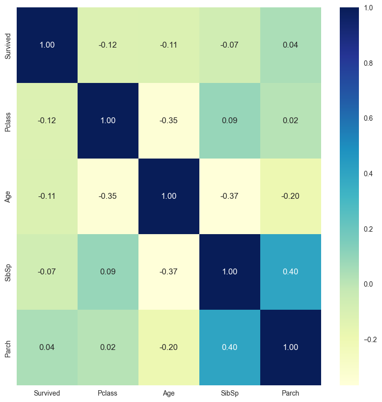
const       28.227667
Survived     1.061895
Pclass       1.173788
Age          1.361584
SibSp        1.351837
Parch        1.199945
dtype: float64get_correlation_by_threshold
get_correlation_by_threshold (df_corr, min_thres=0.98)
| Type | Default | Details | |
|---|---|---|---|
| df_corr | Correlation DataFrame | ||
| min_thres | float | 0.98 | minimum correlation to take |
get_correlation_by_threshold(df_num.corr(),min_thres=0){'Pclass': {'Survived': -0.11633986928104582},
'Age': {'Survived': -0.11211373025858094, 'Pclass': -0.3451575619176082},
'SibSp': {'Survived': -0.06694288369258686,
'Pclass': 0.08741953046914279,
'Age': -0.3664840343129444},
'Parch': {'Survived': 0.03943462980865732,
'Pclass': 0.016490845192711254,
'Age': -0.19765444198507792,
'SibSp': 0.39904002232194297}}get_correlation_by_threshold(df_num.corr(),min_thres=0.3){'Age': {'Pclass': -0.3451575619176082},
'SibSp': {'Age': -0.3664840343129444},
'Parch': {'SibSp': 0.39904002232194297}}plot_cat_correlation
plot_cat_correlation (df_cat, figsize=(10, 10))
| Type | Default | Details | |
|---|---|---|---|
| df_cat | DataFrame with categorical features that have been processed | ||
| figsize | tuple | (10, 10) | Matplotlib figsize |
Let’s process some of the categorical features
from sklearn.preprocessing import OrdinalEncoderfor c in ['Sex','Embarked']:
oe= OrdinalEncoder()
df[c] = oe.fit_transform(df[c].values.reshape(-1,1))df_cat = df[['Survived','Pclass','Sex','Embarked']]df_cat.head()| Survived | Pclass | Sex | Embarked | |
|---|---|---|---|---|
| 0 | 0 | 3 | 1.0 | 2.0 |
| 1 | 1 | 1 | 0.0 | 0.0 |
| 2 | 1 | 3 | 0.0 | 2.0 |
| 3 | 1 | 1 | 0.0 | 2.0 |
| 4 | 0 | 3 | 1.0 | 2.0 |
Cramer’s V measures association between two nominal variables.
Cramer’s V lies between 0 and 1 (inclusive). - 0 indicates that the two variables are not linked by any relation. - 1 indicates that there exists a strong association between the two variables.
plot_cat_correlation(df_cat,(5,5))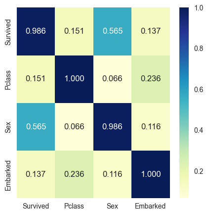
cat_corr = get_cat_correlation(df_cat)
get_correlation_by_threshold(cat_corr,min_thres=0.2)
{'Sex': {'Survived': 0.5650175790296367},
'Embarked': {'Pclass': 0.23572003899034383}}Evaluation plot for regression problem
plot_residuals
 plot_residuals (model, X_trn, y_trn, X_test=None, y_test=None,
                 qqplot=True)
| Type | Default | Details | |
|---|---|---|---|
| model | Regression model | ||
| X_trn | Training dataframe | ||
| y_trn | Training label | ||
| X_test | NoneType | None | Testing dataframe |
| y_test | NoneType | None | Testing label |
| qqplot | bool | True | To whether plot the qqplot |
df_reg = pd.read_csv('http://www.statsci.org/data/general/uscrime.txt',sep='\t')from sklearn.linear_model import LinearRegressionreg_model = LinearRegression()
reg_model.fit(df_reg.drop('Crime',axis=1), df_reg.Crime.values)LinearRegression()In a Jupyter environment, please rerun this cell to show the HTML representation or trust the notebook.
On GitHub, the HTML representation is unable to render, please try loading this page with nbviewer.org.
LinearRegression()
plot_residuals(reg_model, df_reg.drop('Crime',axis=1), df_reg.Crime.values,
X_test=None, y_test=None, qqplot=True)/home/quan/miniforge3/envs/ml_dev/lib/python3.11/site-packages/sklearn/base.py:493: UserWarning: X does not have valid feature names, but LinearRegression was fitted with feature names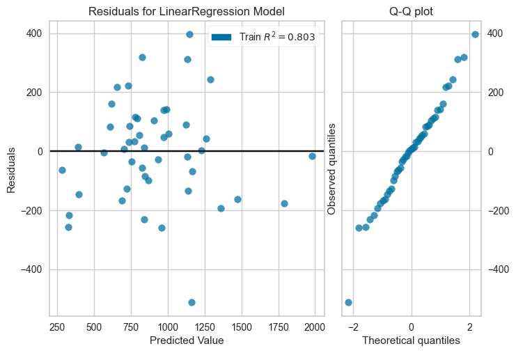
from sklearn.model_selection import train_test_splitX_train, X_test, y_train, y_test = train_test_split(df_reg.drop('Crime',axis=1), df_reg.Crime.values,
test_size=0.2, random_state=42)plot_residuals(reg_model, X_train,y_train,X_test, y_test, qqplot=True)/home/quan/miniforge3/envs/ml_dev/lib/python3.11/site-packages/sklearn/base.py:493: UserWarning: X does not have valid feature names, but LinearRegression was fitted with feature names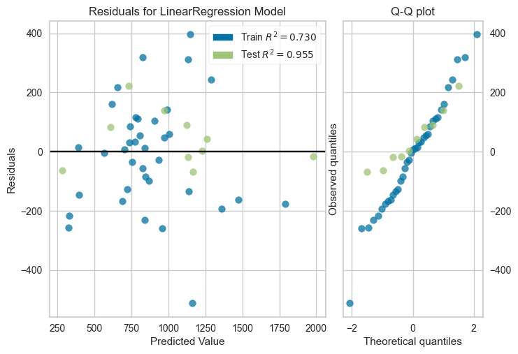
plot_prediction_distribution
plot_prediction_distribution (y_true, y_pred, figsize=(15, 5))
| Type | Default | Details | |
|---|---|---|---|
| y_true | True label numpy array | ||
| y_pred | Prediction numpy array | ||
| figsize | tuple | (15, 5) | Matplotlib figsize |
reg_model = LinearRegression()
reg_model.fit(df_reg.drop('Crime',axis=1), df_reg.Crime.values)LinearRegression()In a Jupyter environment, please rerun this cell to show the HTML representation or trust the notebook.
On GitHub, the HTML representation is unable to render, please try loading this page with nbviewer.org.
LinearRegression()
y_pred = reg_model.predict(df_reg.drop('Crime',axis=1))
y_true = df_reg.Crime.valuesplot_prediction_distribution(y_true,y_pred)MSE: 28828.633430503334
RMSE: 169.789968580312
MAE: 129.91521266409967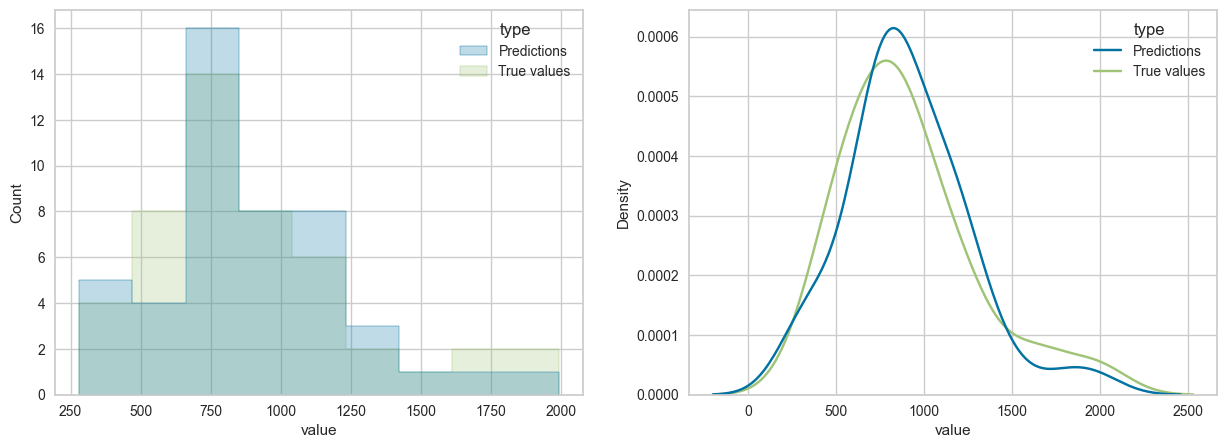
Model evaluation curves
plot_learning_curve
 plot_learning_curve (estimator, title, X, y, axes=None, ylim=None,
                      cv=None, n_jobs=-1, scoring=None, train_sizes=[0.05,
                      0.24, 0.43, 0.62, 0.81, 1.0], save_fig=False,
                      figsize=(20, 5), seed=42)
| Type | Default | Details | |
|---|---|---|---|
| estimator | sklearn’s classifier | ||
| title | Title of the chart | ||
| X | Training features | ||
| y | Training label | ||
| axes | NoneType | None | matplotlib’s axes |
| ylim | NoneType | None | y axis range limit |
| cv | NoneType | None | sklearn’s cross-validation splitting strategy |
| n_jobs | int | -1 | Number of jobs to run in parallel |
| scoring | NoneType | None | metric |
| train_sizes | list | [0.05, 0.24, 0.43, 0.62, 0.81, 1.0] | List of training size portion |
| save_fig | bool | False | To store the chart as png in images directory |
| figsize | tuple | (20, 5) | Matplotlib figsize |
| seed | int | 42 | Random seed |
dt = DecisionTreeClassifier(criterion='entropy',random_state=42,min_samples_leaf=1)
plot_learning_curve(dt,'Learning Curve - Decision Tree - Titanic',df_num.drop('Survived',axis=1),df_num['Survived'],
                      cv=5,scoring='f1_macro',train_sizes=np.linspace(0.1,1,20))
plot_validation_curve
 plot_validation_curve (estimator, title, X, y, ylim=None, cv=None,
                        param_name=None, param_range=None, is_log=False,
                        n_jobs=-1, scoring=None, save_fig=False,
                        figsize=(8, 4), fill_between=True,
                        enumerate_x=False)
| Type | Default | Details | |
|---|---|---|---|
| estimator | sklearn’s classifier | ||
| title | Title of the chart | ||
| X | Training features | ||
| y | Training label | ||
| ylim | NoneType | None | y axis range limit |
| cv | NoneType | None | sklearn’s cross-validation splitting strategy |
| param_name | NoneType | None | Name of model’s hyperparameter |
| param_range | NoneType | None | List containing range of value for param_name |
| is_log | bool | False | To log the value in param_range, for plotting |
| n_jobs | int | -1 | Number of jobs to run in parallel |
| scoring | NoneType | None | metric |
| save_fig | bool | False | To store the chart as png in images directory |
| figsize | tuple | (8, 4) | Matplotlib figsize |
| fill_between | bool | True | To add a upper and lower one-std line for train and test curve |
| enumerate_x | bool | False | Convert categorical hyperparam to numerical, for x axis |
dt = DecisionTreeClassifier(criterion='entropy',random_state=42)
plot_validation_curve(dt,'Val Curve - Decision Tree - Titanic',df_num.drop('Survived',axis=1),df_num['Survived'],
                      cv=5,param_range=np.arange(1,20,1),param_name='max_depth',scoring='f1_macro')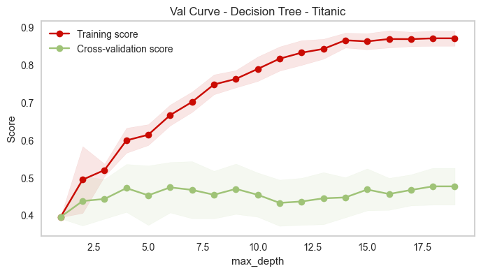
Tree visualization
plot_tree_dtreeviz
 plot_tree_dtreeviz (estimator, X, y, target_name:str,
                     class_names:list=None, tree_index=0,
                     depth_range_to_display=None, fancy=False, scale=1.0)
Plot a decision tree using dtreeviz. Note that you need to install graphviz before using this function
| Type | Default | Details | |
|---|---|---|---|
| estimator | sklearn’s classifier | ||
| X | Training features | ||
| y | Training label | ||
| target_name | str | The (string) name of the target variable; e.g., for Titanic, it’s “Survived” | |
| class_names | list | None | List of names associated with the labels (same order); e.g. [‘no’,‘yes’] |
| tree_index | int | 0 | Index (from 0) of tree if model is an ensemble of trees like a random forest. |
| depth_range_to_display | NoneType | None | Range of depth levels to be displayed. The range values are inclusive |
| fancy | bool | False | To draw fancy tree chart (as opposed to simplified one) |
| scale | float | 1.0 | Scale of the chart. Higher means bigger |
dt = DecisionTreeClassifier(criterion='entropy',random_state=42,class_weight=None,max_depth=3)
dt.fit(df_num.drop('Survived',axis=1),df_num['Survived'])
DecisionTreeClassifier(criterion='entropy', max_depth=3, random_state=42)In a Jupyter environment, please rerun this cell to show the HTML representation or trust the notebook.
On GitHub, the HTML representation is unable to render, please try loading this page with nbviewer.org.
DecisionTreeClassifier(criterion='entropy', max_depth=3, random_state=42)
After you have installed graphviz (https://github.com/parrt/dtreeviz#installation), run these codes to run dtreeviz
plot_tree_dtreeviz(dt,df_num.drop('Survived',axis=1),df_num['Survived'],
                   target_name='Survived',
                   class_names=['no','yes'],
                   fancy=True,scale=1)
/home/quan/miniforge3/envs/ml_dev/lib/python3.11/site-packages/sklearn/base.py:493: UserWarning: X does not have valid feature names, but DecisionTreeClassifier was fitted with feature namesplot_tree_dtreeviz(dt,df_num.drop('Survived',axis=1),df_num['Survived'],
target_name='Survived',
class_names=['no','yes'],
depth_range_to_display=[2,3],
fancy=True,scale=1.2)/home/quan/miniforge3/envs/ml_dev/lib/python3.11/site-packages/sklearn/base.py:493: UserWarning: X does not have valid feature names, but DecisionTreeClassifier was fitted with feature namesplot_classification_tree_sklearn
 plot_classification_tree_sklearn (estimator, feature_names,
                                   class_names:list, rotate=True,
                                   fname='tmp')
Plot a decision tree classifier using sklearn. Note that this will output a png file with fname instead of showing it in the notebook
| Type | Default | Details | |
|---|---|---|---|
| estimator | sklearn’s classifier | ||
| feature_names | List of names of dependent variables (features) | ||
| class_names | list | List of names associated with the labels (same order); e.g. [‘no’,‘yes’] | |
| rotate | bool | True | To rotate the tree graph |
| fname | str | tmp | Name of the png file to save(no extension) |
# feature names (not including label)
feature_names = df_num.drop('Survived',axis=1).columns.values
print(feature_names)
['Pclass' 'Age' 'SibSp' 'Parch']After you have installed graphviz (https://github.com/parrt/dtreeviz#installation), run these codes to run sklearn tree plotting
dt = DecisionTreeClassifier(criterion='entropy',random_state=42,class_weight=None,max_depth=3)
dt.fit(df_num.drop('Survived',axis=1),df_num['Survived'])
plot_tree_sklearn(dt,feature_names=df_num.drop('Survived',axis=1).columns.values,
                  class_names=['no','yes'],
                  rotate=True,fname='tree_depth_3_titanic')
To show the image in notebook, create a markdown cell and type 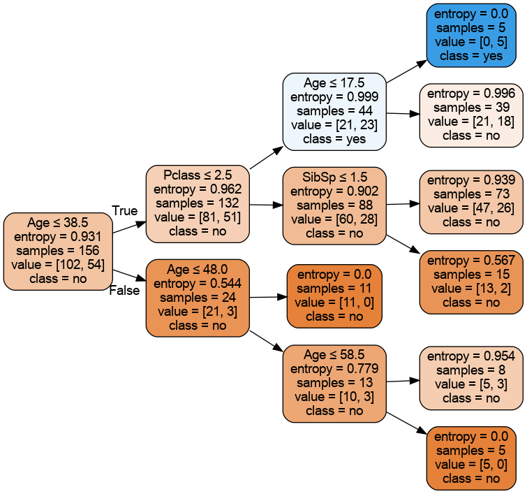

Decision Tree’s feature importances
plot_feature_importances
 plot_feature_importances (importances, feature_names, figsize=(20, 10),
                           top_n=None)
Plot and return a dataframe of feature importances, using sklearn’s feature_importances_ value
| Type | Default | Details | |
|---|---|---|---|
| importances | feature importances from sklearn’s feature_importances_ variable | ||
| feature_names | List of names of dependent variables (features) | ||
| figsize | tuple | (20, 10) | Matplotlib figsize |
| top_n | NoneType | None | Show top n features |
feature_names = df_num.drop('Survived',axis=1).columns.valuesdt = DecisionTreeClassifier(criterion='entropy',random_state=42,class_weight=None,max_depth=5)
dt.fit(df_num.drop('Survived',axis=1),df_num['Survived'])
plot_feature_importances(dt.feature_importances_,feature_names,top_n=3)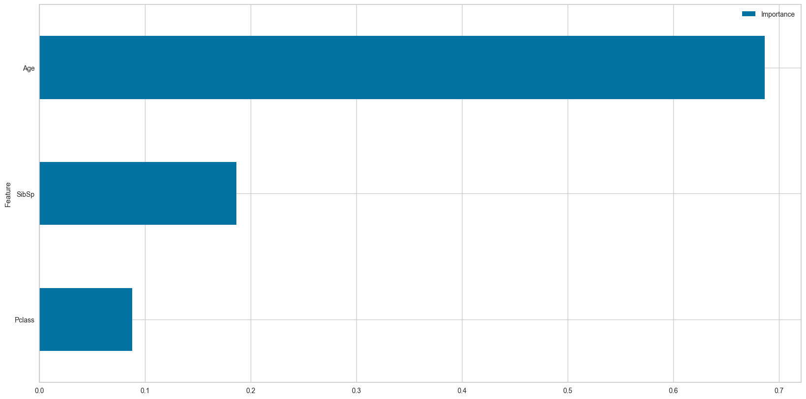
| Importance | |
|---|---|
| Feature | |
| Pclass | 0.087868 |
| SibSp | 0.186577 |
| Age | 0.686647 |
feature_names = df_num.drop('Survived',axis=1).columns.values
dt = DecisionTreeClassifier(criterion='entropy',random_state=42,class_weight=None,max_depth=5)
dt.fit(df_num.drop('Survived',axis=1),df_num['Survived'])

plot_permutation_importances(dt,
                             df_num.drop('Survived',axis=1),
                             df_num['Survived'],
                             scoring=['f1_macro','accuracy'],
                             top_n=3)
f1_macro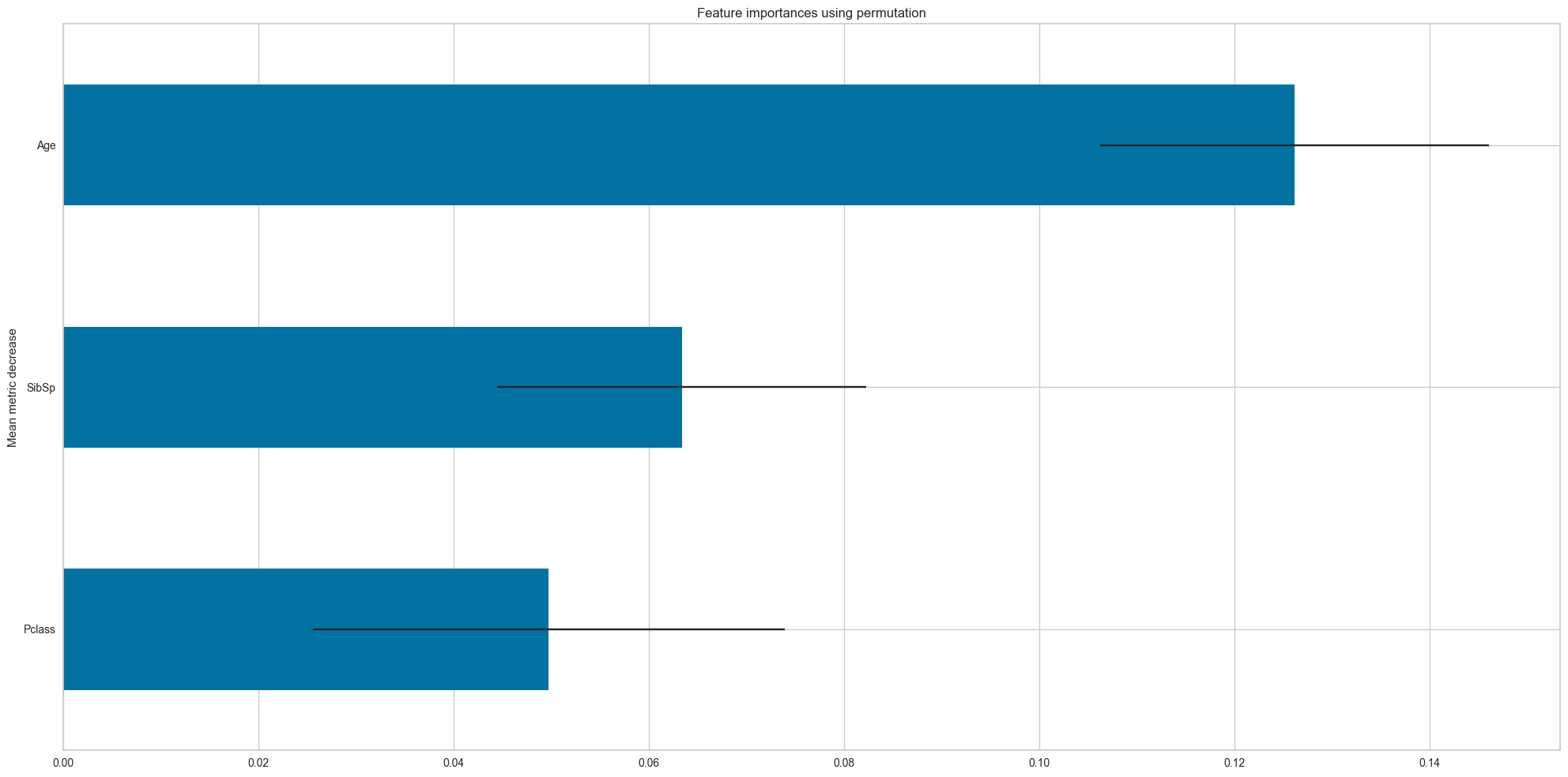
accuracy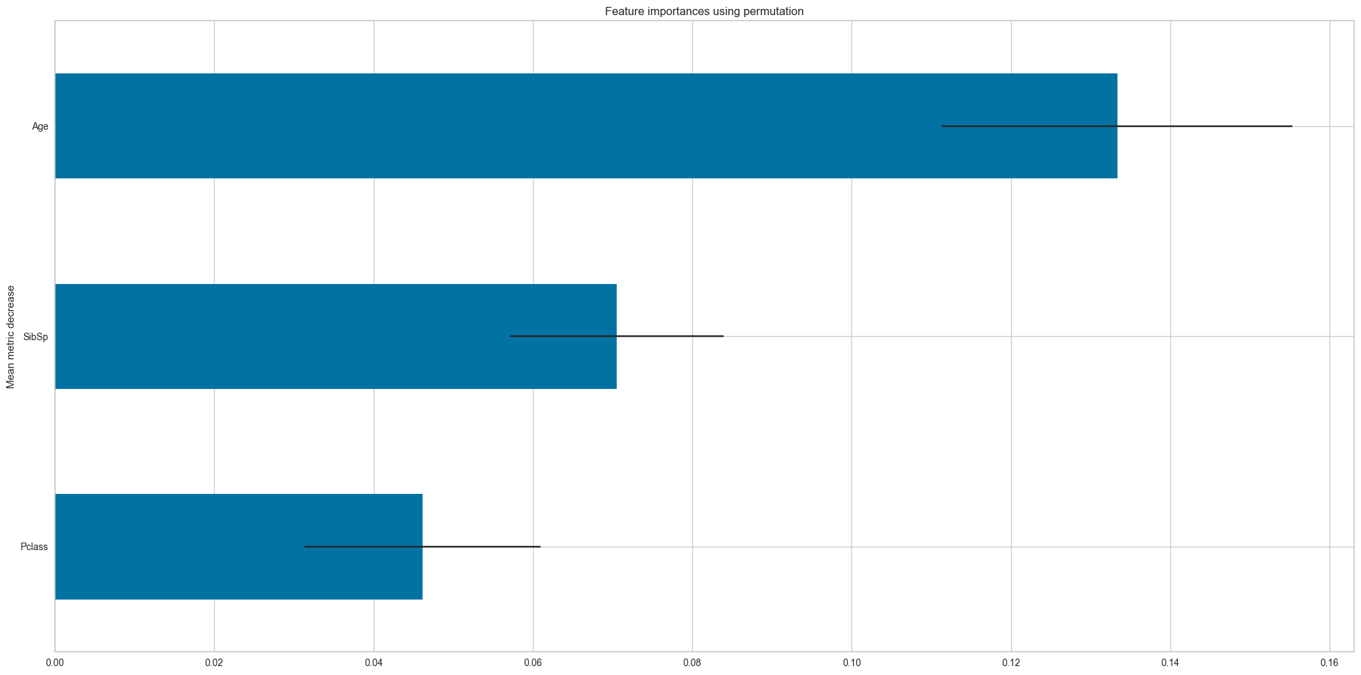
[         Importance       STD
 Feature
 Pclass     0.049733  0.024178
 SibSp      0.063374  0.018909
 Age        0.126187  0.019904,
          Importance       STD
 Feature
 Pclass     0.046154  0.014841
 SibSp      0.070513  0.013446
 Age        0.133333  0.021983]
feature_names = df_num.drop('Survived',axis=1).columns.values
dt = DecisionTreeClassifier(criterion='entropy',random_state=42,class_weight=None,max_depth=5)
dt.fit(df_num.drop('Survived',axis=1),df_num['Survived'])
plot_permutation_importances(dt,
df_num.drop('Survived',axis=1),
df_num['Survived'],
scoring='f1_macro'
)f1_macro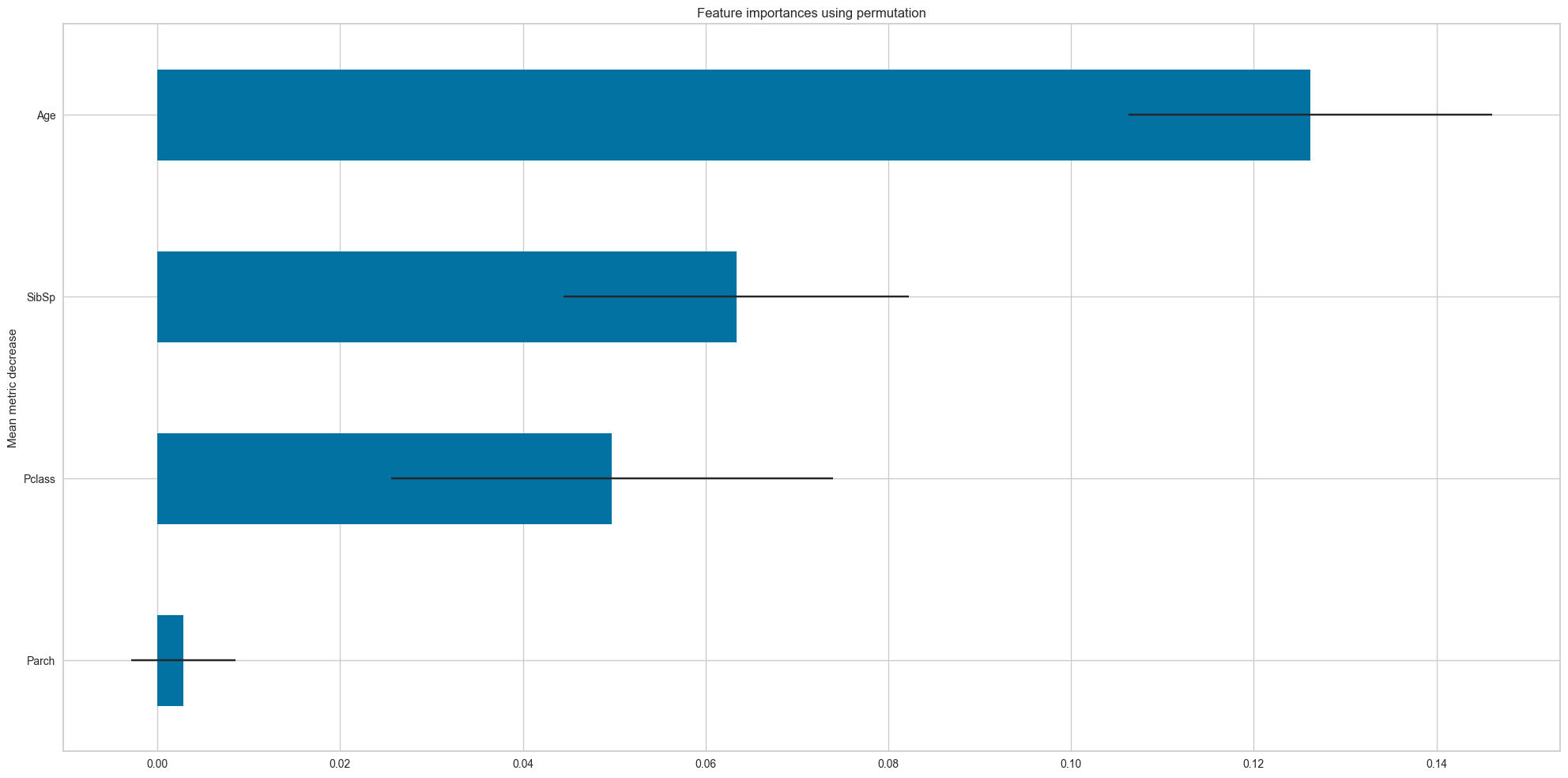
[         Importance       STD
 Feature
 Parch      0.002853  0.005706
 Pclass     0.049733  0.024178
 SibSp      0.063374  0.018909
 Age        0.126187  0.019904]
Hyperparameters visualization
params_2D_heatmap
 params_2D_heatmap (search_cv:dict, param1:str, param2:str,
                    scoring:str='f1_macro', log_param1=False,
                    log_param2=False, figsize=(20, 10), min_hm=None,
                    max_hm=None, higher_is_better=True)
Plot 2D graph of metric value for each pair of hyperparameters
| Type | Default | Details | |
|---|---|---|---|
| search_cv | dict | A dict with keys as column headers and values as columns. Typically an attribute (cv_results_) of GridSearchCV or RandomizedSearchCV | |
| param1 | str | Name of the first hyperparameter | |
| param2 | str | Name of the second hyperparameter | |
| scoring | str | f1_macro | Metric name |
| log_param1 | bool | False | To log the first hyperparameter |
| log_param2 | bool | False | To log the second hyperparameter |
| figsize | tuple | (20, 10) | Matplotlib figsize |
| min_hm | NoneType | None | Minimum value for the metric to show |
| max_hm | NoneType | None | Maximum value of the metric to show |
| higher_is_better | bool | True | Set if high metric is better |
dt = RandomForestClassifier(random_state=42)
param_grid={
    'n_estimators': np.arange(2,20),
    'min_samples_leaf': np.arange(1,80),
}
# Note: in order to use params_2D_heatmap, you should set scoring to a list, and set refit to False
clf = RandomizedSearchCV(dt,param_grid,n_iter=100,
                         scoring=['f1_macro'],n_jobs=-1,
                         cv=5,verbose=1,random_state=42,refit=False)
clf.fit(df_num.drop('Survived',axis=1),df_num['Survived'])
Fitting 5 folds for each of 100 candidates, totalling 500 fits/home/quan/miniforge3/envs/ml_dev/lib/python3.11/site-packages/numpy/ma/core.py:2820: RuntimeWarning: invalid value encountered in castRandomizedSearchCV(cv=5, estimator=RandomForestClassifier(random_state=42),
n_iter=100, n_jobs=-1,
param_distributions={'min_samples_leaf': array([ 1, 2, 3, 4, 5, 6, 7, 8, 9, 10, 11, 12, 13, 14, 15, 16, 17,
18, 19, 20, 21, 22, 23, 24, 25, 26, 27, 28, 29, 30, 31, 32, 33, 34,
35, 36, 37, 38, 39, 40, 41, 42, 43, 44, 45, 46, 47, 48, 49, 50, 51,
52, 53, 54, 55, 56, 57, 58, 59, 60, 61, 62, 63, 64, 65, 66, 67, 68,
69, 70, 71, 72, 73, 74, 75, 76, 77, 78, 79]),
'n_estimators': array([ 2, 3, 4, 5, 6, 7, 8, 9, 10, 11, 12, 13, 14, 15, 16, 17, 18,
19])},
random_state=42, refit=False, scoring=['f1_macro'],
verbose=1)In a Jupyter environment, please rerun this cell to show the HTML representation or trust the notebook. On GitHub, the HTML representation is unable to render, please try loading this page with nbviewer.org.
RandomizedSearchCV(cv=5, estimator=RandomForestClassifier(random_state=42),
                   n_iter=100, n_jobs=-1,
                   param_distributions={'min_samples_leaf': array([ 1,  2,  3,  4,  5,  6,  7,  8,  9, 10, 11, 12, 13, 14, 15, 16, 17,
       18, 19, 20, 21, 22, 23, 24, 25, 26, 27, 28, 29, 30, 31, 32, 33, 34,
       35, 36, 37, 38, 39, 40, 41, 42, 43, 44, 45, 46, 47, 48, 49, 50, 51,
       52, 53, 54, 55, 56, 57, 58, 59, 60, 61, 62, 63, 64, 65, 66, 67, 68,
       69, 70, 71, 72, 73, 74, 75, 76, 77, 78, 79]),
                                        'n_estimators': array([ 2,  3,  4,  5,  6,  7,  8,  9, 10, 11, 12, 13, 14, 15, 16, 17, 18,
       19])},
                   random_state=42, refit=False, scoring=['f1_macro'],
verbose=1)RandomForestClassifier(random_state=42)
RandomForestClassifier(random_state=42)
params_2D_heatmap(clf.cv_results_,'n_estimators','min_samples_leaf',
                  scoring='f1_macro',
                  figsize=(20,10))
/tmp/ipykernel_16177/2399879344.py:14: MatplotlibDeprecationWarning: The get_cmap function was deprecated in Matplotlib 3.7 and will be removed two minor releases later. Use ``matplotlib.colormaps[name]`` or ``matplotlib.colormaps.get_cmap(obj)`` instead.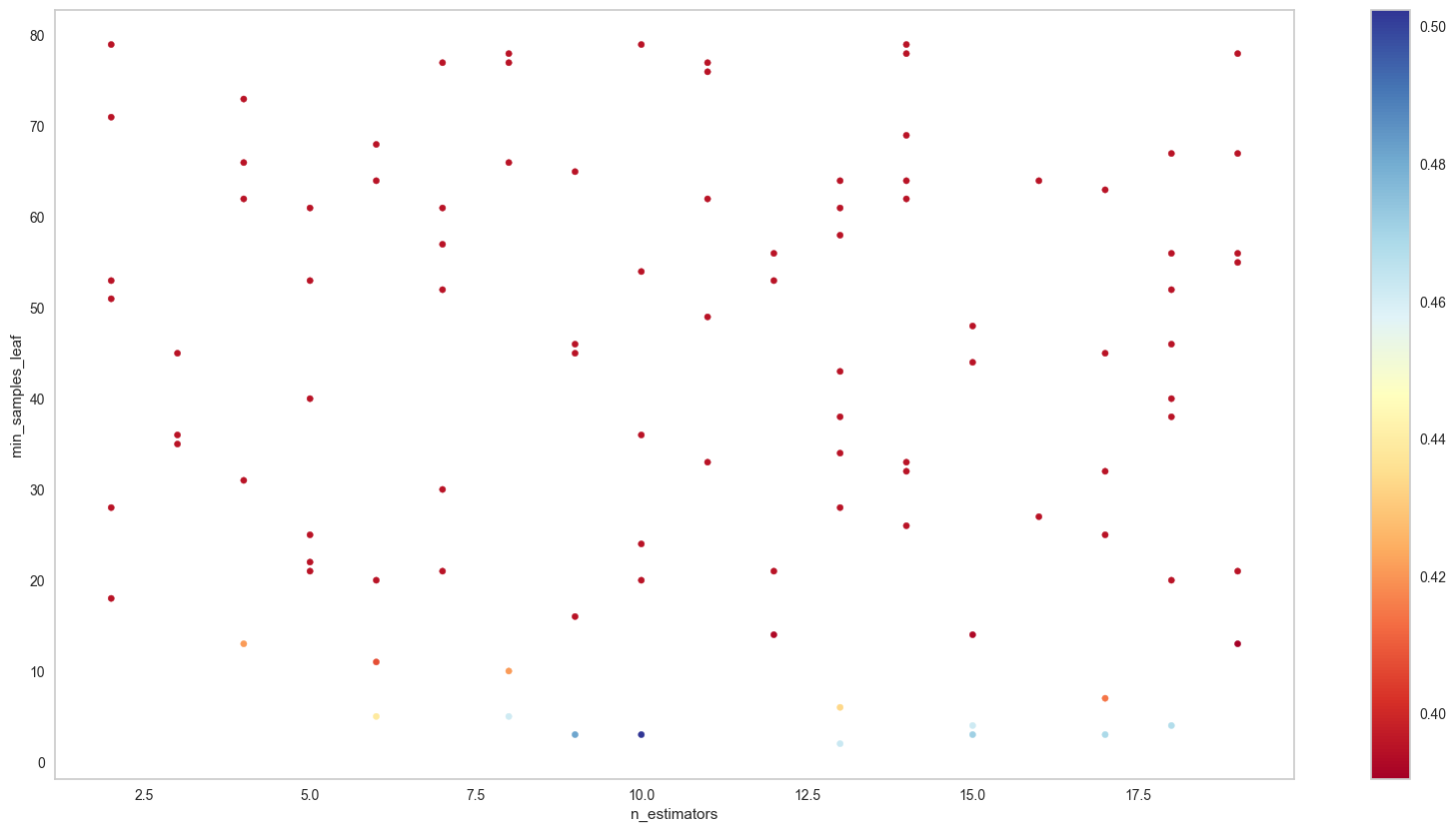
params_2D_heatmap(clf.cv_results_,'n_estimators','min_samples_leaf',
                  scoring='f1_macro',
                  figsize=(20,10),min_hm=0.45)
/tmp/ipykernel_16177/2399879344.py:14: MatplotlibDeprecationWarning: The get_cmap function was deprecated in Matplotlib 3.7 and will be removed two minor releases later. Use ``matplotlib.colormaps[name]`` or ``matplotlib.colormaps.get_cmap(obj)`` instead.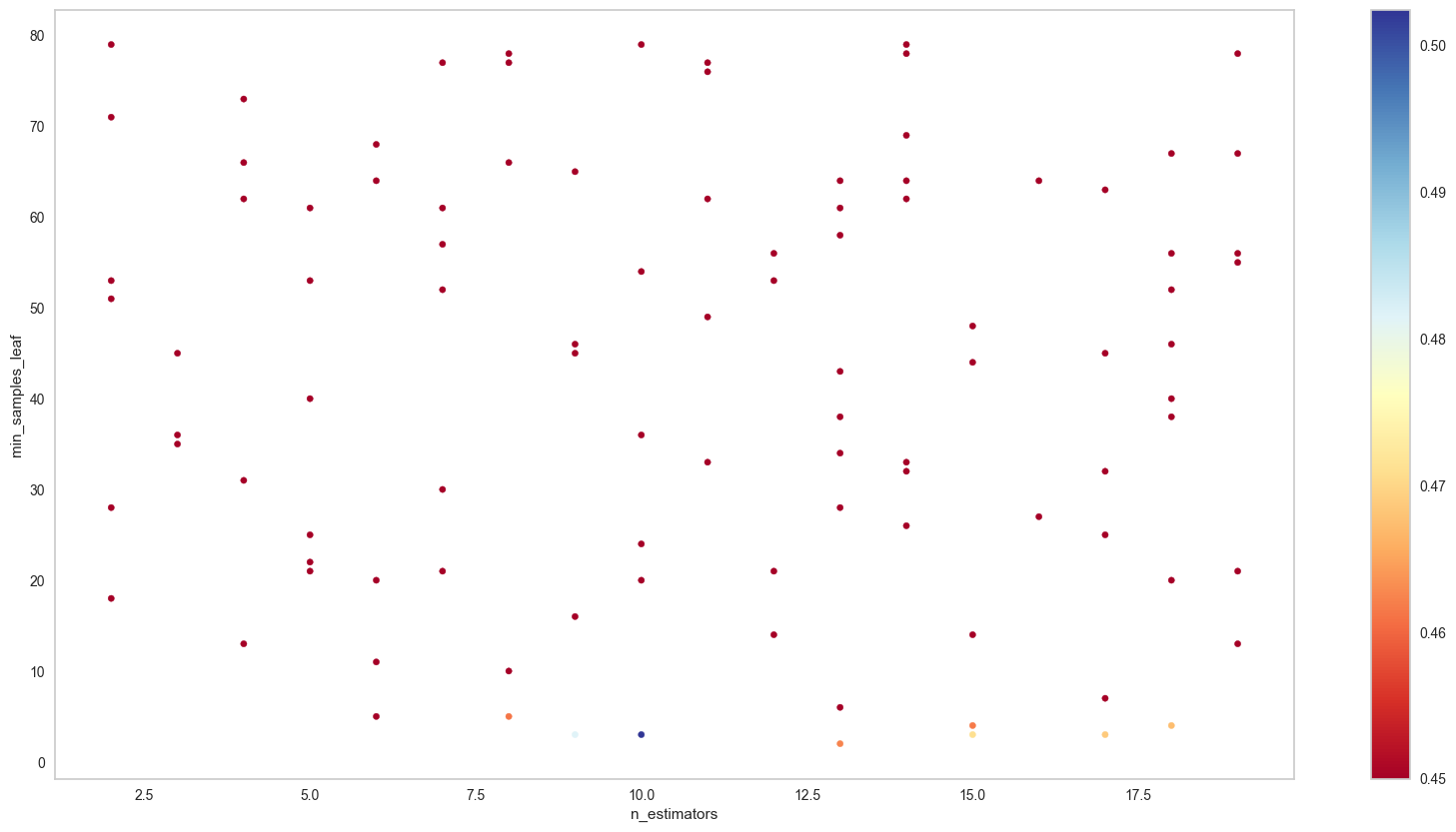
dt = RandomForestClassifier(random_state=42)
param_grid={
    'n_estimators': np.arange(2,20),
    'min_samples_leaf': np.arange(1,80),
    'max_features': [0.3,0.4,0.5,0.6,0.7,0.8,0.9,1],
}
# Note: in order to use params_2D_heatmap, you should set scoring to a list, and set refit to False
clf = RandomizedSearchCV(dt,param_grid,n_iter=100,
                         scoring=['f1_macro'],n_jobs=-1,
                         cv=5,verbose=1,random_state=42,refit=False)
clf.fit(df_num.drop('Survived',axis=1),df_num['Survived'])
Fitting 5 folds for each of 100 candidates, totalling 500 fitsRandomizedSearchCV(cv=5, estimator=RandomForestClassifier(random_state=42),
n_iter=100, n_jobs=-1,
param_distributions={'max_features': [0.3, 0.4, 0.5, 0.6,
0.7, 0.8, 0.9, 1],
'min_samples_leaf': array([ 1, 2, 3, 4, 5, 6, 7, 8, 9, 10, 11, 12, 13, 14, 15, 16, 17,
18, 19, 20, 21, 22, 23, 24, 25, 26, 27, 28, 29, 30, 31, 32, 33, 34,
35, 36, 37, 38, 39, 40, 41, 42, 43, 44, 45, 46, 47, 48, 49, 50, 51,
52, 53, 54, 55, 56, 57, 58, 59, 60, 61, 62, 63, 64, 65, 66, 67, 68,
69, 70, 71, 72, 73, 74, 75, 76, 77, 78, 79]),
'n_estimators': array([ 2, 3, 4, 5, 6, 7, 8, 9, 10, 11, 12, 13, 14, 15, 16, 17, 18,
19])},
random_state=42, refit=False, scoring=['f1_macro'],
verbose=1)In a Jupyter environment, please rerun this cell to show the HTML representation or trust the notebook. On GitHub, the HTML representation is unable to render, please try loading this page with nbviewer.org.
RandomizedSearchCV(cv=5, estimator=RandomForestClassifier(random_state=42),
                   n_iter=100, n_jobs=-1,
                   param_distributions={'max_features': [0.3, 0.4, 0.5, 0.6,
                                                         0.7, 0.8, 0.9, 1],
                                        'min_samples_leaf': array([ 1,  2,  3,  4,  5,  6,  7,  8,  9, 10, 11, 12, 13, 14, 15, 16, 17,
       18, 19, 20, 21, 22, 23, 24, 25, 26, 27, 28, 29, 30, 31, 32, 33, 34,
       35, 36, 37, 38, 39, 40, 41, 42, 43, 44, 45, 46, 47, 48, 49, 50, 51,
       52, 53, 54, 55, 56, 57, 58, 59, 60, 61, 62, 63, 64, 65, 66, 67, 68,
       69, 70, 71, 72, 73, 74, 75, 76, 77, 78, 79]),
                                        'n_estimators': array([ 2,  3,  4,  5,  6,  7,  8,  9, 10, 11, 12, 13, 14, 15, 16, 17, 18,
       19])},
                   random_state=42, refit=False, scoring=['f1_macro'],
verbose=1)RandomForestClassifier(random_state=42)
RandomForestClassifier(random_state=42)
params_3D_heatmap(clf.cv_results_,
                  'n_estimators',
                  'min_samples_leaf',
                  'max_features',
                  scoring='f1_macro')
Partial Dependency Plot
pdp_numerical_only
 pdp_numerical_only (model, X:pandas.core.frame.DataFrame,
                     num_features:list, class_names:list, y_colors=None,
                     ncols=2, nrows=2, figsize=(20, 16))
Plot PDP plot for numerical dependent variables
| Type | Default | Details | |
|---|---|---|---|
| model | sklearn tree model that has been trained | ||
| X | pd.DataFrame | dataframe to perform pdp | |
| num_features | list | A list of numerical features | |
| class_names | list | List of names associated with the labels (same order); e.g. [‘no’,‘yes’] | |
| y_colors | NoneType | None | List of colors associated with class_names |
| ncols | int | 2 | |
| nrows | int | 2 | |
| figsize | tuple | (20, 16) |
df = pd.read_csv('https://raw.githubusercontent.com/plotly/datasets/master/titanic.csv')
df = df[['Survived','Pclass','Sex','Age','SibSp','Parch','Embarked']].copy()
df = preprocessing_general(df,
                           missing_cols=['Age','Embarked'],
                           missing_vals=np.NaN,
                           strategies=['median','most_frequent'],
                           cat_cols='Embarked',
                           bi_cols='Sex'
)df.head()| Survived | Pclass | Age | SibSp | Parch | Embarked_C | Embarked_Q | Embarked_S | Sex_male | |
|---|---|---|---|---|---|---|---|---|---|
| 0 | 0 | 3 | 22.0 | 1 | 0 | 0.0 | 0.0 | 1.0 | 1.0 |
| 1 | 1 | 1 | 38.0 | 1 | 0 | 1.0 | 0.0 | 0.0 | 0.0 |
| 2 | 1 | 3 | 26.0 | 0 | 0 | 0.0 | 0.0 | 1.0 | 0.0 |
| 3 | 1 | 1 | 35.0 | 1 | 0 | 0.0 | 0.0 | 1.0 | 0.0 |
| 4 | 0 | 3 | 35.0 | 0 | 0 | 0.0 | 0.0 | 1.0 | 1.0 |
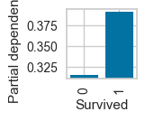
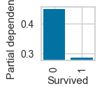
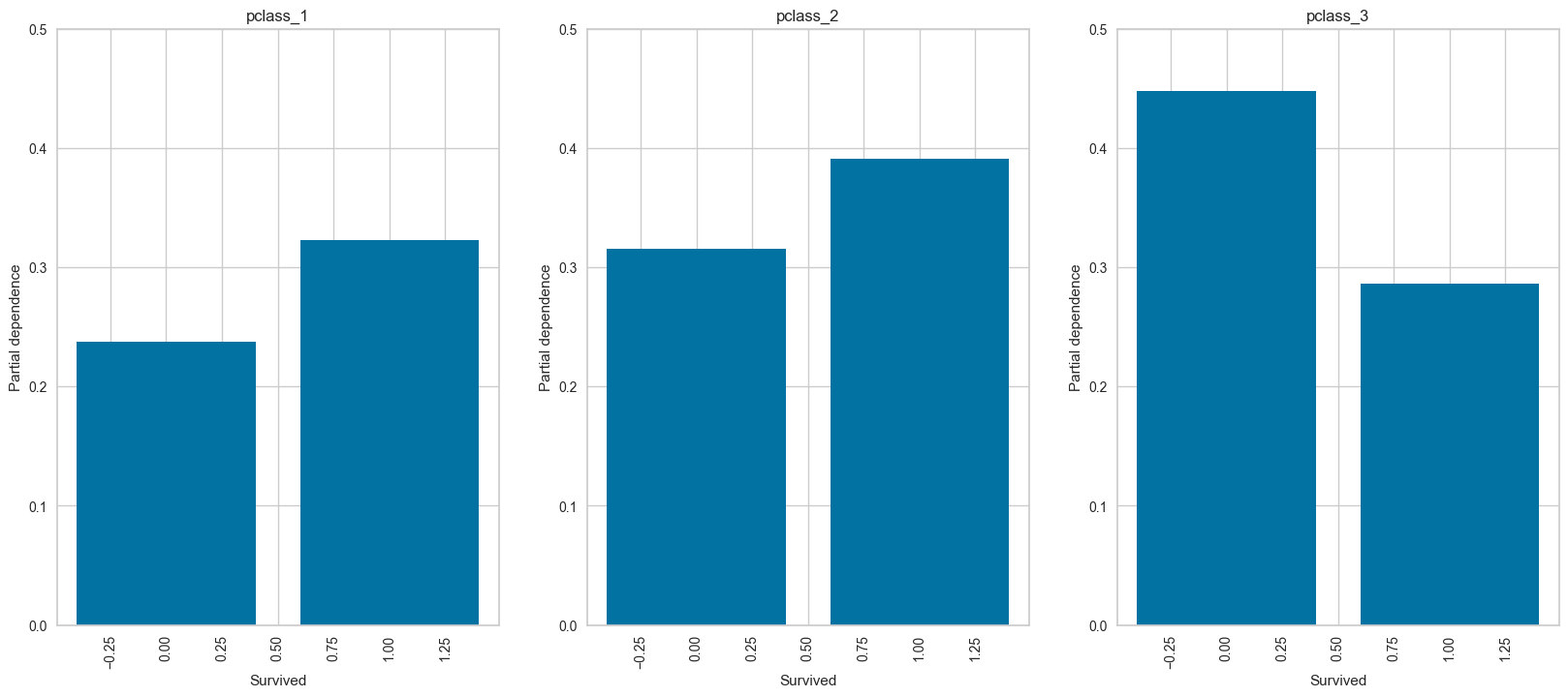
To better showcase the interpretation of Partial Dependency Plot, we will reuse the Titanic dataset, but now the independent variable (the one we need to predict) will be Pclass (3 classes to predict)
params = {'n_estimators': 12, 'min_samples_leaf': 10, 'max_features': 0.8, 'class_weight': 'balanced'}
X_trn = df.drop('Pclass',axis=1)
y_trn = LabelEncoder().fit_transform(df['Pclass'])
dt = RandomForestClassifier(**params)
dt.fit(X_trn,y_trn)
RandomForestClassifier(class_weight='balanced', max_features=0.8,
min_samples_leaf=10, n_estimators=12)In a Jupyter environment, please rerun this cell to show the HTML representation or trust the notebook. On GitHub, the HTML representation is unable to render, please try loading this page with nbviewer.org.
RandomForestClassifier(class_weight='balanced', max_features=0.8,
min_samples_leaf=10, n_estimators=12)pdp_numerical_only(dt,X_trn,num_features=['Age','SibSp'],class_names=['pclass_1','pclass_2','pclass_3'],nrows=2,ncols=1,figsize=(6,8))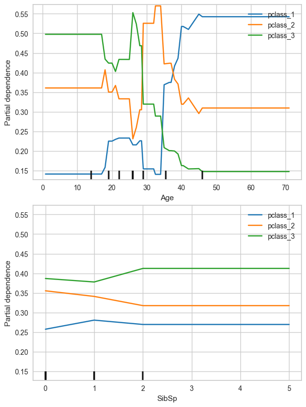
pdp_categorical_only
 pdp_categorical_only (model, X:pandas.core.frame.DataFrame,
                       cat_feature:list, class_names:list, y_colors=None,
                       ymax=0.5, figsize=(20, 8))
Plot PDP plot for categorical dependent variables
| Type | Default | Details | |
|---|---|---|---|
| model | sklearn tree model that has been trained | ||
| X | pd.DataFrame | dataframe to perform pdp | |
| cat_feature | list | A single categorical feature | |
| class_names | list | List of names associated with the labels (same order); e.g. [‘no’,‘yes’] | |
| y_colors | NoneType | None | List of colors associated with class_names |
| ymax | float | 0.5 | |
| figsize | tuple | (20, 8) |
pdp_categorical_only(dt,X_trn,'Survived',
                     class_names=['pclass_1','pclass_2','pclass_3'])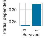
plot_ice_pair
 plot_ice_pair (model, X:pandas.core.frame.DataFrame, pair_features:list,
                class_idx, figsize=(10, 4))
Plot ICE plot from a pair of numerical feature
| Type | Default | Details | |
|---|---|---|---|
| model | sklearn tree model that has been trained | ||
| X | pd.DataFrame | dataframe to perform ice | |
| pair_features | list | a list of only 2 features | |
| class_idx | index of the class to plot | ||
| figsize | tuple | (10, 4) |
# For pclass_1
plot_ice_pair(dt,X_trn,pair_features=['Age','SibSp'],class_idx=0,figsize=(8,3))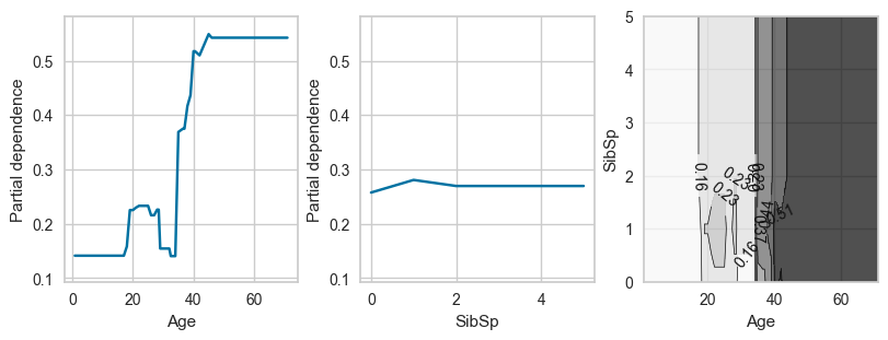
# For pclass_2
plot_ice_pair(dt,X_trn,pair_features=['Age','SibSp'],class_idx=1,figsize=(8,3))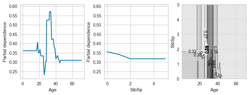
# For pclass_3
plot_ice_pair(dt,X_trn,pair_features=['Age','SibSp'],class_idx=2,figsize=(8,3))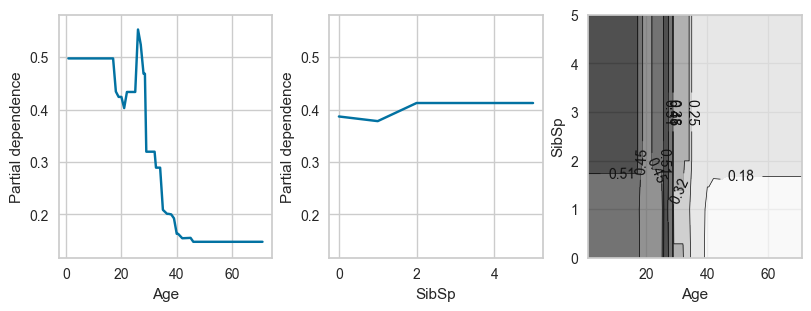
Other functions
plot_confusion_matrix
 plot_confusion_matrix (y_true:list|numpy.ndarray,
                        y_pred:list|numpy.ndarray, labels=None)
Simple function to plot the confusion matrix
| Type | Default | Details | |
|---|---|---|---|
| y_true | list | np.ndarray | A list/numpy array of true labels | |
| y_pred | list | np.ndarray | A list/numpy array of predictions | |
| labels | NoneType | None | Display names matching the labels (same order). |
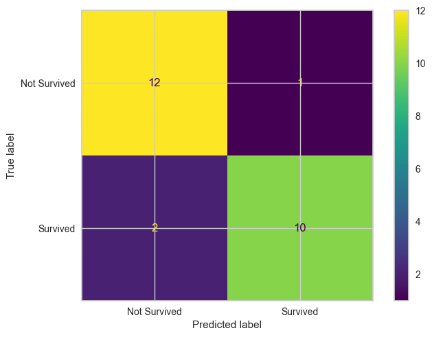
y_true = np.array([1, 1, 1, 0, 0, 1, 1, 0, 1, 1, 1, 0, 0, 0, 0, 1, 0, 0, 1, 1, 0, 0, 1, 0, 0])
y_pred = np.array([1, 0, 1, 0, 0, 1, 1, 0, 0, 1, 1, 0, 0, 0, 0, 1, 0, 0, 1, 1, 1, 0, 1, 0, 0])plot_confusion_matrix(y_true,y_pred,labels=['Not Survived','Survived'])